The Fed Anchors the Short End, Not Your Mortgage

One regression, three targets. The 2-year Treasury is cointegrated with the policy rate; the 30-year mortgage is not — and the difference is the whole story.

Executive summary

Regressing the 30-year fixed mortgage rate on the effective federal funds rate (monthly, Jan 2000 – Dec 2024, n = 300) yields R² = 0.656 and t = 23.8. Both figures are misleading.
A unit root in the residuals cannot be rejected ( p = 0.087), and the two series are (Engle–Granger p = 0.224). That is the signature of a in the Granger–Newbold sense: two persistent series drifting together, not a stable relationship.
Applying the identical method to the 2-year Treasury gives a different answer. That pair is cointegrated (p = 0.0002), its residuals are stationary, and its rolling coefficient never turns negative in 25 years. The mortgage’s does — it reaches −4.77.
Put the 10-year Treasury in the model and the fed funds coefficient collapses to 0.005 (t = 0.1) while R² does not move. The funds rate carries no information about mortgage rates that the long end has not already priced.
Out of sample, the mortgage model is beaten by the most naive benchmark available: expanding-window RMSE of 0.958 versus 0.194 for “next month equals this month.”
The economically coherent reading: the policy rate anchors the short end of the curve, and does not anchor the long end. A 30-year mortgage is priced at the long end.

Key numbers


Sample	Monthly, Jan 2000 – Dec 2024, n = 300
Baseline	Mortgage = 4.080 + 0.558 × fed funds · R² = 0.656
Cointegration, fed funds ↔ 2-year	p = 0.0002 — long-run relationship
Cointegration, fed funds ↔ 30-year mortgage	p = 0.224 — none
Fed funds β, controlling for the 10-year	0.005 (t = 0.1) — adds nothing
Rolling β range, mortgage	−4.77 to +4.86
Out-of-sample RMSE vs no-change	0.958 vs 0.194
Primary caveat	Observational data. Association, not identified causation.

The research question

Every tightening cycle produces the same headline: the Fed is raising mortgage rates. It is a testable claim. If the policy rate drives the cost of home financing, a regression of one on the other should show a stable, economically meaningful relationship that survives basic time-series diagnostics.

This note tests that claim, and then does something the original test did not: it runs the same specification against the 2-year Treasury as a control. If the method is sound, it should behave sensibly on a security the Fed genuinely dominates. It does — which is what makes the mortgage result interesting rather than merely negative.

This began as a university econometrics assignment: regress the 30-year fixed mortgage rate on the effective federal funds rate and interpret the output. The task was narrow, I ran it correctly, and it received full credit.

What sent me back to it was the strength of that output. An R² of 0.656 and a t-statistic near 24 look like a finding, and I wanted to know whether they described a stable economic relationship or simply two persistent rate series drifting through the same broad cycle. The assignment never asked that question. The diagnostics answered it clearly enough that the project stopped being coursework.

Everything past the baseline is new: the stationarity and cointegration testing, and the comparison against the 2-year and 10-year Treasury. None of it was in the original assignment, and the 2-year control is what turned a negative result into a legible one.

Economic framework

The says a longer-term rate is roughly the average expected short rate over its life, plus a . That framing predicts the result found here rather than contradicting it:

The 2-year Treasury is, to a first approximation, the market’s forecast of the average federal funds rate over the next two years, plus a small premium. The Fed does not merely influence it — over a two-year horizon it substantially is it. A tight relationship is close to definitional.
The 30-year mortgage is priced off the 10-year Treasury plus a . The 10-year embeds long-run inflation expectations, growth expectations, and a term premium that the FOMC does not set. The MBS spread moves with and convexity risk, bank funding conditions, origination economics, and the Fed’s balance sheet — none of which is the funds rate.

So the transmission mechanism is real, but it runs through the long end, and the long end has its own drivers. Mortgage rates are not the policy rate plus a fixed spread. Between June 2004 and June 2006 the FOMC raised the funds rate by 396 and the 30-year mortgage moved 39 bp — , and it sits inside this sample.

Data and methodology

Series	FRED ID	Definition	Frequency
Federal funds	`FEDFUNDS`	Effective rate, monthly average	Monthly
30-year mortgage	`MORTGAGE30US`	Freddie Mac PMMS, US average	Weekly → monthly
2-year Treasury	`GS2`	Constant maturity, monthly average	Monthly
10-year Treasury	`GS10`	Constant maturity, monthly average	Monthly

Sample: January 2000 – December 2024, 300 monthly observations, no gaps, no duplicate dates. All series in percent. Estimation in Excel (Data Analysis ToolPak); diagnostics and replication in Python (statsmodels). The baseline was reproduced from the raw spreadsheet data — not copied from the printed output — and matches to seven decimal places.

Inference uses standard errors where reported, because the residuals are both and .

Results

The baseline, as originally estimated:

Mortgage rate = 4.080 + 0.558 × fed funds rate

R² = 0.656 · slope SE = 0.023 · t = 23.8 · F = 568.6 · n = 300

That t is the first thing to go. is 0.067 against a healthy 2.0 — near-perfect serial correlation, which makes the OLS standard errors far too small. Correcting with Newey–West (HAC, 12 lags):

	OLS	HAC-corrected
Slope	0.558	0.558
Std. error	0.023	0.050
t-statistic	23.8	11.2

The point estimate is untouched; roughly half the apparent precision was an artifact of untreated autocorrelation. The slope still clears any conventional bar — which is why the diagnostics below, not the t-statistic, carry the argument.

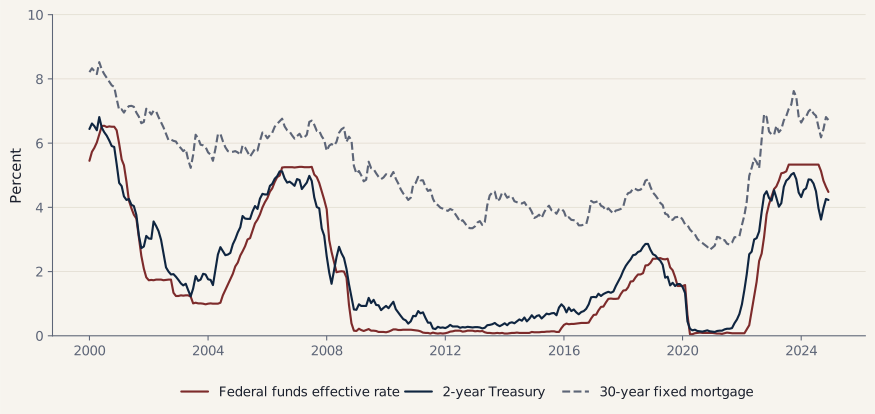
Federal funds rate, 2-year Treasury and 30-year mortgage rate, monthly, 2000 to 2024

Exhibit 1. Federal funds effective rate, 2-year Treasury, and 30-year fixed mortgage rate. Monthly, January 2000 – December 2024, percent. Source: Federal Reserve Bank of St. Louis (FRED): FEDFUNDS, GS2; Freddie Mac MORTGAGE30US. As of Dec 2024. All three move together over the cycle — which is exactly the impression the levels regression formalises, and exactly what the diagnostics below undermine.

The same regression, three targets:

Fed funds →	β	R²	Durbin–Watson	Residual ADF (p)	Cointegration (p)	Verdict
2-year Treasury	0.839	0.918	0.150	0.0000	0.0002	Cointegrated
10-year Treasury	0.485	0.566	0.068	0.092	0.234	Spurious
30-year mortgage	0.558	0.656	0.067	0.087	0.224	Spurious

The 2-year passes. The mortgage does not. Same regressor, same sample, same estimator.

In monthly changes — does a policy move actually pass through?

Fed funds →	β	HAC t	R²
2-year Treasury	0.509	8.0	0.202
30-year mortgage	0.127	2.2	0.014

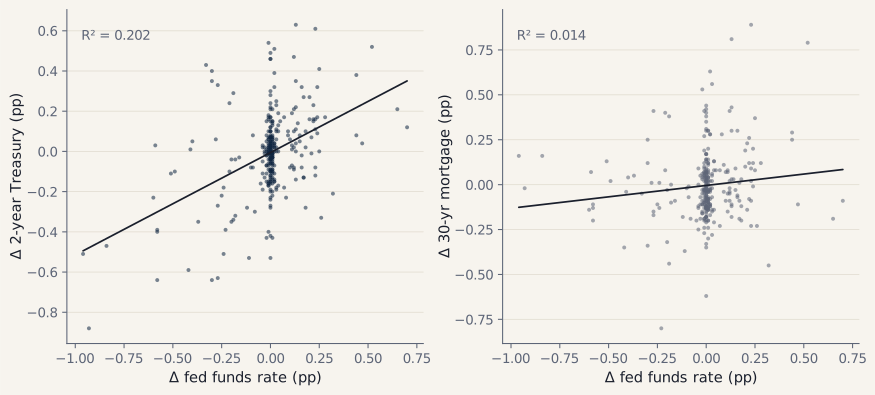
Scatter plots of monthly changes in the 2-year Treasury and in the 30-year mortgage rate against monthly changes in the fed funds rate, with fitted lines

Exhibit 2. Monthly changes in the 2-year Treasury (left) and the 30-year mortgage rate (right) against monthly changes in the federal funds rate, with fitted OLS lines. Percentage points, Jan 2000 – Dec 2024. Source: FRED. HAC (Newey–West, 6 lags). The left panel has a slope you can see; the right is close to a cloud.

Does the funds rate add anything the 10-year doesn’t?

The pass-through coefficient above is small but not zero. The sharper test is whether it survives once the rate the mortgage is actually priced off — the 10-year Treasury — is in the model:

Specification (monthly changes)	R²	Fed funds coefficient
Δ Mortgage ~ Δ FedFunds	0.014	+0.127 (HAC t = 2.2)
Δ Mortgage ~ Δ 10Y	0.707	—
Δ Mortgage ~ Δ 10Y + Δ FedFunds	0.707	+0.005 (t = 0.1)

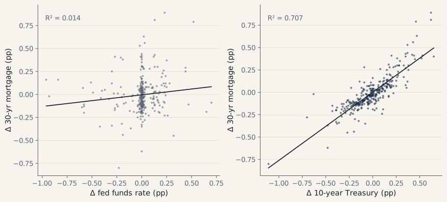
Scatter plots of monthly changes in the 30-year mortgage rate against changes in the fed funds rate and against changes in the 10-year Treasury, with fitted lines

Exhibit 3. Monthly changes in the 30-year mortgage rate against changes in the fed funds rate (left, R² = 0.014) and against changes in the 10-year Treasury (right, R² = 0.707), with fitted OLS lines. Same data, same period, same dependent variable. Source: FRED. HAC (Newey–West, 6 lags).

The third row is the finding. Add the 10-year and the fed funds coefficient falls to 0.005 with t = 0.1 — indistinguishable from zero, while R² does not move at all. The funds rate carries no information about mortgage rates that the 10-year does not already carry.

This also explains why the levels regression looked strong: fed funds and the 10-year correlate 0.75 in levels. The funds rate was standing in for the 10-year.

Robustness and limitations

Parameter stability is where the mortgage model fails hardest.

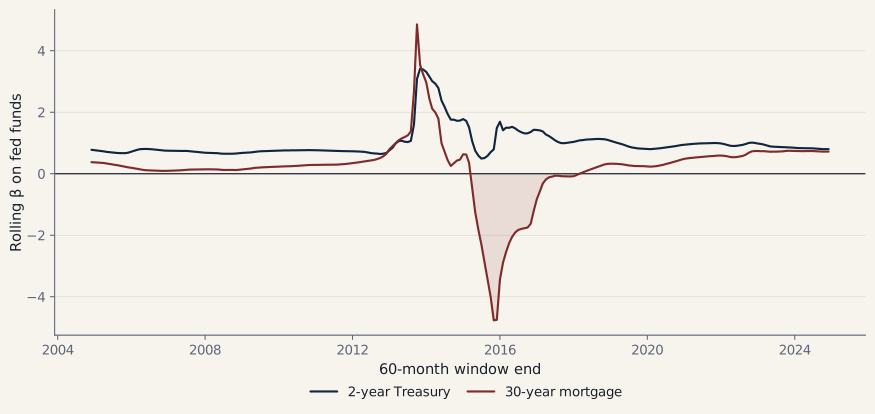
Sixty-month rolling coefficient on the fed funds rate for the 2-year Treasury and for the 30-year mortgage, by window end date

Exhibit 4. Coefficient on the federal funds rate from 60-month rolling regressions, plotted against the window’s end date. Shaded where the mortgage coefficient is negative. Source: FRED; author’s calculations. The 2-year coefficient stays positive in every window of the sample. The mortgage coefficient ranges from −4.77 to +4.86 and is negative in 15% of windows — a range of 9.6 around a full-sample “estimate” of 0.558.

The two episodes that matter most. If the 0.558 pass-through were structural, it should hold in large, sustained tightening cycles. It fails in both in the sample — and fails in opposite directions, which is the signature of a relationship that isn’t there rather than one that is merely mismeasured:

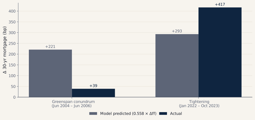
Model-predicted versus actual change in the 30-year mortgage rate across the 2004 to 2006 and 2022 to 2023 tightening cycles

Exhibit 5. Model-predicted versus realised change in the 30-year mortgage rate across the two largest tightening episodes in the sample. Source: FRED; author’s calculations. Predicted = 0.558 × Δ fed funds.

	Fed moved	Model predicted	Actual	Error
Jun 2004 – Jun 2006	+396 bp	+221 bp	+39 bp	−182 bp
Jan 2022 – Oct 2023	+525 bp	+293 bp	+417 bp	+124 bp

The first is Greenspan’s conundrum. A model that misses by 182 bp one way and 124 bp the other way in the next cycle is not describing a mechanism.

Structural breaks. reject stability at three of the four policy dates tested — December 2008 (F = 98.6), December 2015 (F = 90.6) and March 2020 (F = 19.3). The fourth, January 2022, does not reject (F = 0.6): the most recent tightening cycle did not itself break the relationship, it inherited one that was already broken.

Those four dates bound five regimes, and the coefficient is different in every one:

Regime	Window	n	β on fed funds
Pre-GFC	Jan 2000 – Nov 2008	107	0.254
	Dec 2008 – Nov 2015	84	3.674
Normalization	Dec 2015 – Feb 2020	51	0.279
COVID ZLB	Mar 2020 – Dec 2021	22	0.733
Tightening	Jan 2022 – Dec 2024	36	0.478

The full-sample 0.558 describes no actual period. It is an average of five regimes that disagree by more than a factor of ten.

Forecasting. Expanding-window validation (train on everything before t, predict t, no shuffling):

	RMSE	MAE
Regression on fed funds	0.958	0.857
No-change benchmark	0.194	0.133
Historical mean	1.673	1.598

The regression is roughly five times worse than assuming next month looks like this month. Directional accuracy is 55.3%. This model should not be used to forecast, and no forecast is offered here.

On the original point estimate. The baseline implies a 6.50% mortgage rate at a 4.33% funds rate. That number reproduces exactly — but its 95% prediction interval is [4.88%, 8.11%], a 3.2-point range spanning “housing boom” to “housing frozen.” A point estimate without that interval overstates what the model knows.

What is clean. Cook’s distance flags zero influential observations (max 0.0130 against a 4/n threshold of 0.0133). The result is not an artifact of outliers or of a single episode. The problem is the specification, not the data.

What this note does not establish. These are observational data with no identification strategy. Cointegration between the funds rate and the 2-year is a statement about a long-run statistical relationship, not a controlled experiment. The theory is consistent with the finding; it does not convert it into proof of causation.

Market implications

For borrowers: watching FOMC meetings to time a mortgage is watching the wrong variable. The 10-year Treasury and the MBS spread carry the information.
For duration: the short end is anchored to policy and is where policy expectations express themselves cleanly. The long end is not, and treating it as a lagged policy rate will misprice it.
For reading the cycle: a stable policy rate is entirely compatible with large moves in mortgage rates. Those moves come from inflation expectations, term premium and MBS spreads.

Where I’d put weight, and where I wouldn’t.

The 2-year Treasury contains predictive information about the expected policy path. That is closer to definitional than empirical — a 2-year yield is approximately the average federal funds rate the market expects over roughly the next two years, plus a — and the results here are consistent with it. The relationship to the funds rate is materially stronger at the 2-year than at the 10-year or the mortgage. It does not follow that the 2-year anticipates individual FOMC decisions, and I would not use it that way.

On mortgages I’d state it more narrowly. The evidence suggests transmission runs through the long end of the Treasury curve and the rather than from the policy rate directly. The Fed still affects financing conditions — nothing here says otherwise — but the transmission is indirect, variable across regimes, and not one-for-one. A stable policy rate is entirely compatible with large moves in mortgage rates.

The methodological point is the one I’d defend hardest: a high R² in a levels regression is not sufficient evidence of forecasting power. This model explains 66% of the variation in mortgage rates and still loses to “next month equals this month” out of sample by roughly five times. Fit and forecasting are different claims. Only the diagnostics and chronological out-of-sample testing separate them, and they are the part of this note I would run first next time rather than last.

What would change my mind

If the fed funds coefficient held above 0.2 with t > 2 after controlling for the 10-year in a sample excluding the zero-lower-bound years, the “adds nothing” conclusion would need revising.
If the mortgage/fed-funds pair tested cointegrated on a longer sample (1971–2024, spanning Volcker), the spurious-regression verdict would be sample-specific rather than structural.
If an error-correction specification produced stable adjustment coefficients across regimes, the instability shown here would be an artifact of the levels form rather than of the relationship.
If the regression beat a no-change benchmark out of sample at any horizon, the forecasting verdict would change.

Conclusion

The coursework model was correct for what it was asked to do. As an exercise in estimating and interpreting a bivariate regression it was executed properly, and I would run it the same way again for that purpose.

Held to a research standard, it does not survive. A unit root in the residuals cannot be rejected, the two series are not , the coefficient is unstable to the point of changing sign, and out of sample the model loses to the most naive benchmark available. The simple mortgage-levels regression should not be treated as a reliable forecasting model, and I am not treating it as one.

But the strongest finding here is not that the federal funds rate is irrelevant. It is that monetary policy anchors the short end of the curve far more directly than the long end. The 2-year Treasury largely reflects the expected policy path. A 30-year mortgage absorbs that too, and then adds long-run inflation expectations, growth expectations, a term premium the FOMC does not set, and an MBS spread with drivers of its own. Same regressor, same sample, same estimator — and the answer depends almost entirely on where you point it.

That is the part I’d carry forward. Statistical significance is the start of a test, not the end of one. Before a model is used to forecast anything, or to justify a position, it has to survive the diagnostics that ask whether the relationship it describes is stable and real. This one didn’t — and establishing that was worth more than the original result was.

Methodology appendix

Baseline. OLS, levels: MORTGAGE30US ~ α + β·FEDFUNDS. n = 300. Reproduced from raw data: Multiple R 0.810015, R² 0.656124, Adj R² 0.654970, SE 0.818204, intercept 4.079982, β 0.557938 (SE 0.023398), t 23.845, F 568.591, Significance F 4.78 × 10⁻⁷¹. ANOVA: SS regression 380.6477 (df 1), SS residual 199.4986 (df 298), SS total 580.1463 (df 299). 95% CI on β: [0.512, 0.604].

On the intercept. 4.080 is the model’s fitted value at a zero funds rate within this sample. It is not a structural “natural” mortgage rate, and the sample contains only the 2009–15 and 2020–21 episodes near zero to inform it.

Diagnostics. Durbin–Watson 0.067; residual AR(1) 0.966; Ljung–Box rejects at lags 1, 6, 12 (p < 1e-60). Breusch–Pagan p = 0.002 and White p = 2.2e-09 (heteroskedastic). Jarque–Bera p = 0.012 (skew 0.291, kurtosis 2.396). ADF: FEDFUNDS stationary (p = 0.001), MORTGAGE30US non-stationary (p = 0.223); KPSS agrees on both. Regressing an I(1) series on an I(0) series is unbalanced. Engle–Granger: mortgage p = 0.224, 2-year p = 0.0002.

Robustness. First differences; 3-lag distributed lag (cumulative 4-month pass-through 0.172, no individual lag significant); multiple regression including GS10; 60-month rolling windows; Chow tests at four policy dates; five regime subsamples; expanding-window out-of-sample validation against no-change and historical-mean benchmarks.

Specifications, stated so the figures above can be reproduced rather than taken on trust. Cointegration is Engle–Granger with the target regressed on the funds rate — the test is not symmetric, and reversing the arguments changes the mortgage p-value from 0.224 to 0.070. Residual AR(1) is the lag-1 autocorrelation of the residual series (0.9664), consistent with the 1 − DW/2 approximation. Regime subsamples are bounded by the Chow break dates, not by calendar years: pre-GFC is Jan 2000 – Nov 2008, the zero-lower-bound era is Dec 2008 – Nov 2015, and the tightening cycle is Jan 2022 – Dec 2024. Out-of-sample validation uses a 120-month burn-in and then expands one month at a time — train on everything strictly before t, predict t, never shuffle — giving 180 chronological predictions. Directional accuracy compares the sign of the change in the model’s prediction against the sign of the change in the realised rate, on the same 180 predictions.

Reproducibility. Every series is public and free from FRED — no paid data, no API key. Both workbooks are downloadable:

Original regression workbook (.xlsx) — the estimation as first run, in Excel, unmodified.
Methodology workbook (.xlsx) — README, raw data, baseline (live formulas), diagnostics, robustness, and sources.

Sources

Board of Governors of the Federal Reserve System. Federal Funds Effective Rate [FEDFUNDS]. FRED, Federal Reserve Bank of St. Louis. https://fred.stlouisfed.org/series/FEDFUNDS
Freddie Mac. 30-Year Fixed Rate Mortgage Average in the United States [MORTGAGE30US]. FRED. https://fred.stlouisfed.org/series/MORTGAGE30US
Board of Governors. Market Yield on U.S. Treasury Securities at 2-Year Constant Maturity [GS2]. FRED. https://fred.stlouisfed.org/series/GS2
Board of Governors. Market Yield on U.S. Treasury Securities at 10-Year Constant Maturity [GS10]. FRED. https://fred.stlouisfed.org/series/GS10
Bernanke, Ben S., and Alan S. Blinder. “The Federal Funds Rate and the Channels of Monetary Transmission.” American Economic Review, vol. 82, no. 4, 1992, pp. 901–921.
Granger, C.W.J., and P. Newbold. “Spurious Regressions in Econometrics.” Journal of Econometrics, vol. 2, no. 2, 1974, pp. 111–120.
Engle, Robert F., and C.W.J. Granger. “Co-Integration and Error Correction: Representation, Estimation, and Testing.” Econometrica, vol. 55, no. 2, 1987, pp. 251–276.
Newey, Whitney K., and Kenneth D. West. “A Simple, Positive Semi-Definite, Heteroskedasticity and Autocorrelation Consistent Covariance Matrix.” Econometrica, vol. 55, no. 3, 1987, pp. 703–708.

This note revises an earlier version of my own analysis — a university econometrics assignment from March 2026 — which reported the levels regression without stationarity or autocorrelation diagnostics and concluded that changes in the funds rate “reliably translate” into mortgage costs. The data does not support that conclusion, and this note supersedes it. The assignment contained the baseline regression only; the diagnostics, the cointegration testing and the Treasury comparisons are new work.

Ken Capital is an independent investment-research portfolio. This note is personal research and not investment advice. Estimation sample ends December 2024; no current-market values are stated.